Robert F. Bourque, Ph. D., P.E.
Bourque Engineering LLC
Los Alamos, New Mexico USA
bob@rfbourque.net
505-412-0194
Chapter |
Title |
1 |
|
2 |
|
3 |
|
4 |
|
5 |
|
6 |
|
7 |
|
8 |
|
9 |
|
10 |
|
11 |
|
12 |
|
13 |
|
14 |
|
15 |
|
16 |
|
17 |
|
18 |
|
19 |
|
20 |
|
21 |
|
|
|
|
|
|
A Compact Pollution-Free
External Combustion Engine
with High Part-Load Efficiency
Previous Chapter | Next Chapter
10. First Example Engine in a Vehicle
Several examples are given below of engines in specified vehicles. These vehicles were used in the software written by the author to estimate performance. They were specified either by weight and coastdown runs performed by the author to get the road power curve, or by weight, frontal area, and drag coefficient that was used in a standard formula.
|
|
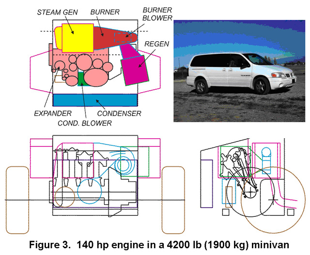
Figure 3 shows the first example, a 104 kW (140 hp) engine, as it would be installed in the author’s 1900 kg (4200 lb) minivan. Shown are the two Burners, Steam Generator, Expander, Regenerator, two Blowers, and Condenser. The Expander, which is discussed in detail later, is a tilted ‘V’ configuration, making it look odd in the top view. Also shown is the outline of the existing transaxle. This presented a challenge because it takes up considerable engine compartment space. (With rear-wheel drive it is behind the engine compartment and out of the way.) Nevertheless, as seen, the front-wheel-drive engine does fit.
One interesting item, shown in tan at the bottom, is a braking blower. To compensate for lack of compression braking, an air blower can be attached to the Expander. Air flow through it is zero until the brakes are applied. Then air is admitted to provide the equivalent drag as compression braking.
|
|
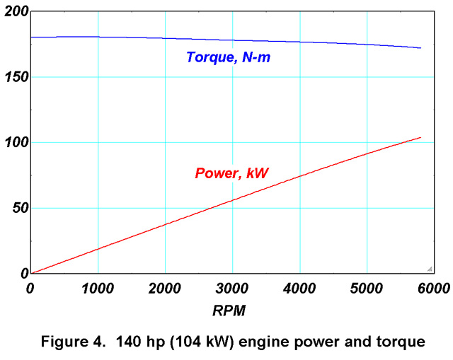
Figure 4 shows the calculated power and torque for this engine at wide-open throttle. The very flat torque curve permits reduced peak power for a given overall performance. The slight dropoff is due to increasing pressure drops and mechanical friction as engine speed is increased.
|
|
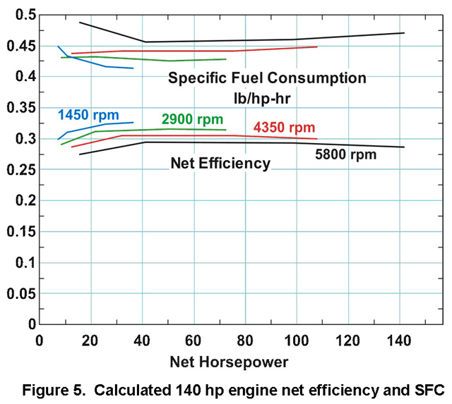
Figure 5 shows calculated net efficiency and specific fuel consumption (SFC) with gasoline. Although any fuel can be used, these plots have been made using the most familiar fuels: gasoline for cars, and diesel for trucks, buses and locomotives.
The right ends of the curves in Figure 5 indicate power at wide-open throttle at that rpm. As seen, net efficiency is about 28% at maximum full power. Although quite good, it gets even better: It increases at lower speeds and throttle settings, reaching 32% at half speed and 33% at quarter speed. Specific fuel consumption is between 0.42 and 0.47 lb/hp-hr (256-286 gm/kW-hr) at normal load settings. The odd jump in SFC at 1450 rpm appears to be from software convergence tolerance.
|
|
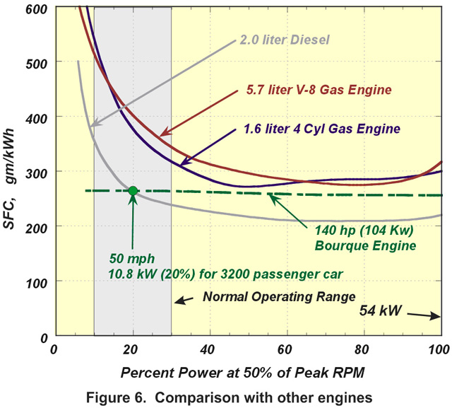
These results are compared in Figure 6 to IC engines, taken from a variety of sources [12,13,14]. The curves show SFC for 50% rpm. This time the steam engine is installed in a 1452 kg (3200 lb) passenger car. In that vehicle the engine needs to supply 25 kW or less at steady speed. The 10.8 kW shows how little power is needed to propel it on a level road at 80 km/hr (50 mph). Note that the two gas engines, shown in red and blue, have around 50% higher SFC in the normal operating range (lower SFC is better). Only the diesel matches the steam engine. This suggests that passenger vehicles should have about 50% higher fuel economy if their gas engine were replaced with this engine. Replacing diesel engines should give about the same fuel economy but would have cleaner burning, multifuel capability, and quieter operation.
|
|
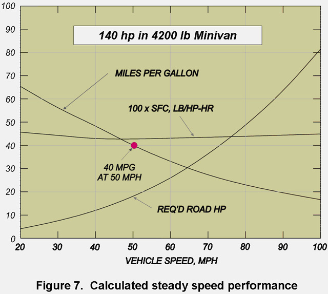
Figure 7 shows calculated steady-speed perform-ance of the 140 hp engine in the minivan. The road power curve was determined from extensive coastdown runs. As seen, miles per gallon is very sensitive to speed, which reflects the fact that engine efficiency increases with decreasing load.
|
|
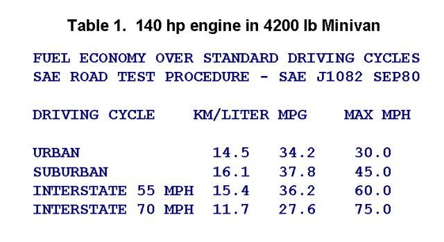
Of course, steady speed results do not reflect actual driving. For this reason, the software written by the author includes the SAE Standard Driving Cycles. These cycles include starts and stops, and acceleration to speed, as well as periods of steady speed. Table 1 shows calculated fuel economy, taken from the code output, over the four SAE Driving Cycles. As seen, fuel economy is very high even under these conditions. These values compare very favorably with the nominal 9.3-10.6 km/l (22-25 mpg) reported by owners [15] and by the author.
|
|
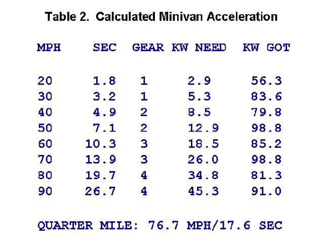
The engines have been sized to provide enough power for good acceleration for a street vehicle. It also provides for ample grade climbing. Table 2 shows code output of acceleration for the minivan. A four-speed torque convertor is used. Although fewer speeds would work because of the flat torque curve, a transmission is still needed to get high power, that comes only at the high rpm’s, to the ground at low vehicle speed. The instantaneous accelerating force equals the surplus power (KW GOT - KW NEED in the table) divided by the vehicle velocity.